Read UV-Vis Spectra in Your Browser: λmax, Beer–Lambert, Colour and Tauc Band Gaps
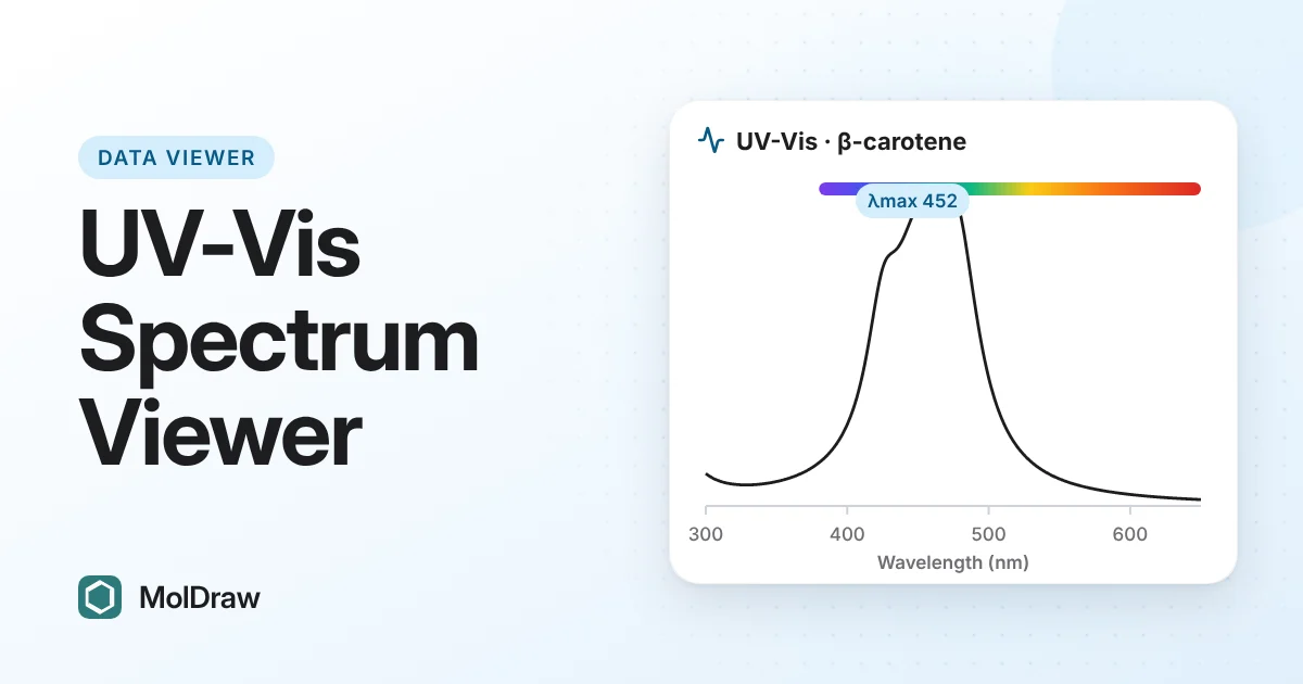
Short answer: Open a JCAMP-DX or CSV/TXT file in the free MolDraw UV-Vis viewer, or press an example such as β-Carotene. The viewer lists the λmax peaks, works out ε or concentration from A = εcl, names the colour the sample shows, overlays a series and fits a Tauc plot for a band gap. It runs in your browser, and your files stay on your device.
Try the UV-Vis viewer here
Why use a browser viewer for UV-Vis data?
UV-Vis is one of the quickest measurements in a lab. The slow part comes after: you have a file and need λmax, a molar absorptivity, a figure or a band gap. In a spreadsheet that means converting units, finding maxima by eye and building plots by hand. The viewer does these steps on one page, with nothing to install.
The science in brief
λmax. Molecules absorb UV and visible light when an electron moves to a higher orbital, as in π→π* or n→π* transitions. λmax is the wavelength where a band absorbs most. Longer conjugation moves it to longer wavelengths. β-carotene, with eleven conjugated C=C bonds, absorbs in the blue part of the visible range.
To get a rough idea of where a compound should absorb before you measure it, predict UV-Vis bands from a drawn structure with the Spectroscopy plugin.
Beer–Lambert law. Absorbance is A = εcl, where ε is the molar absorptivity (L mol⁻¹ cm⁻¹), c the concentration (mol/L) and l the path length (cm). Also, A = −log10T. The law holds best for dilute solutions.
Colour. A sample looks the colour complementary to the light it absorbs. A band in the blue makes a solution look yellow. A band in the green, as in permanganate, makes it look purple.
Tauc plot. For a semiconductor, plot (αhν)2 against photon energy hν for a direct allowed transition, or (αhν)1/2 for an indirect allowed one. Extend the straight part of the absorption edge to zero. The crossing point estimates the optical band gap, Eg.
Files you can open
- JCAMP-DX (.jdx, .dx). The viewer reads the x and y units from the file.
- CSV or TXT with two columns. The x column can be in nm, µm, cm⁻¹ or eV. The y column can be absorbance or transmittance. Without headers, the viewer guesses from the numbers.
Pick several files at once to overlay them. To practise, use the simulated examples or download the sample .jdx.
How to analyse a spectrum, step by step
- Press Open UV-Vis file(s) or drop files on the box. You can also press an example: β-Carotene, KMnO4, Dye series (5 conc.), ZnO band gap or Sample .jdx file.
- Choose Absorbance or %T for the y axis, and nm, eV or cm⁻¹ for the x axis.
- Read the λmax peaks table. It gives each peak in nm, eV and cm⁻¹ with its absorbance and colour. Move the Peak prominence slider if a shoulder is missing or small bumps show up.
- In the Beer-Lambert box, enter Path l (cm) and a Concentration in mol/L, mmol/L or µmol/L to get ε and log ε. Or enter ε to get the concentration. Tap a table row or the plot to use another wavelength. Use λmax again switches back.
- For a band gap, open Tauc plot and band gap, choose the Transition, and press Auto fit or type your own Fit from (eV) and to values.
- Press Export PNG, Export CSV or Tauc PNG.
What the viewer does
| Peaks | Up to eight maxima for the selected spectrum, largest first. |
|---|---|
| Beer–Lambert | ε and log ε from a concentration, or concentration from ε, at λmax or a wavelength you tap. A warning appears above A = 1.5. |
| Colour | The colour of the strongest visible band (380 to 780 nm), from a standard colour wheel. |
| Overlay | Several spectra in different colours, each with a show box, and an option to normalise each to its maximum. |
| Tauc plot | Direct or indirect, automatic or manual fit range, Eg in eV and nm, and R². |
| Export | PNG of the spectrum or Tauc plot, and CSV of the visible spectra in the current units. |
Ways to use it in class and in the lab
- Conjugation and colour: load β-Carotene, then add KMnO4 with Add to the plot instead of replacing. Compare where each absorbs and why one looks yellow and the other purple.
- Checking Beer–Lambert: load the dye series. Select each spectrum by its name and enter its concentration. If the law holds, ε should come out about the same each time.
- Unknown concentration: enter ε from a calibration or the literature to get c.
- Semiconductor films: use the ZnO example to learn the Tauc method, then open your own film spectrum. For an organic semiconductor, compare that optical gap with the electrochemical gap from HOMO and LUMO estimates in the cyclic voltammetry viewer.
- Lab reports: export a PNG for the figure and a CSV for the data.
Tips and limits
- Record a solvent blank on the spectrometer. The viewer does not subtract one.
- A weak shoulder on a large band may not appear as a peak.
- The Tauc plot uses absorbance in place of the absorption coefficient α. This is fine for finding where the line meets zero. For powders measured by diffuse reflectance, convert to the Kubelka–Munk function before you open the file.
- Check the shaded fit range and R² before you report Eg. Another range can give another answer.
- The colour is a guide. Real colour also depends on band width, concentration and the light source.
- The CSV puts all visible spectra on the x values of the first one, so spectra with different grids are interpolated.
Questions and answers
What absorbance range gives reliable Beer–Lambert results?
Aim for absorbances between about 0.1 and 1. Above 1.5 very little light reaches the detector, stray light matters and the line bends, so the viewer shows a warning. Dilute the sample or use a shorter cell.
Why does a sample that absorbs blue light look yellow?
We see the light that is not absorbed. If a band removes blue light from white light, the rest looks yellow, the complementary colour on the colour wheel.
Should I use a direct or an indirect Tauc plot?
Use the transition type known for your material. ZnO, for example, has a direct gap and silicon an indirect one. If the type is not known, say which plot you used when you report the band gap.
Can I use the viewer with unpublished data?
Yes. The page reads and draws your files in the browser, so the files stay on your device.