Computational Chemistry Add-on: Open Gaussian and ORCA Files in Your Browser
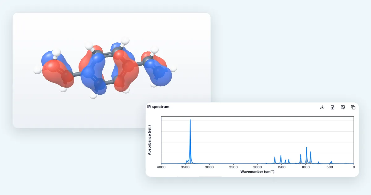
Short answer: Open the 3D viewer, press + and install Computational Chemistry. In the CompChem tab, drop a Gaussian, ORCA, GAMESS, xtb, Molden, cube or trajectory file (or open an example). You get the key results, IR/Raman and UV-Vis spectra you can export or copy as transparent images, animated normal modes, molecular orbitals, trajectories with energy profiles, and a builder for your next input file.
How to read the screenshots: each orange number in a picture matches the numbered note under it. Dashed boxes with a magnified panel are zoomed-in details.
Step 1: Install the Computational Chemistry add-on
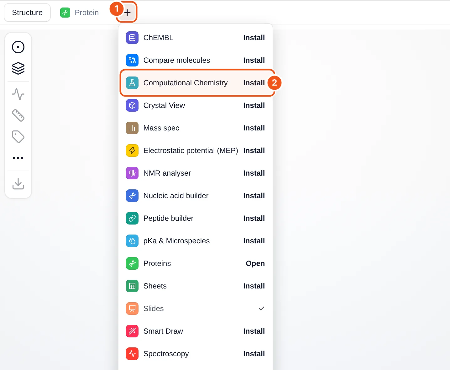
- The + button at the end of the tab row (Structure, Protein, …) opens the add-on menu.
- Computational Chemistry: click Install and a CompChem tab appears.
- Open the MolDraw editor and sign in. A free account is enough to use add-ons.
- Open the 3D viewer on the right (the 3D button at the bottom of the atom bar) and press + next to the tabs.
- Click Install next to Computational Chemistry (callout 2). The CompChem tab opens, and the button changes to Open.
Add-ons stay installed on your account. To remove one, hover its tab and click the small ×. You can also manage them under Settings › Plugins.
Step 2: Open an output file or an example
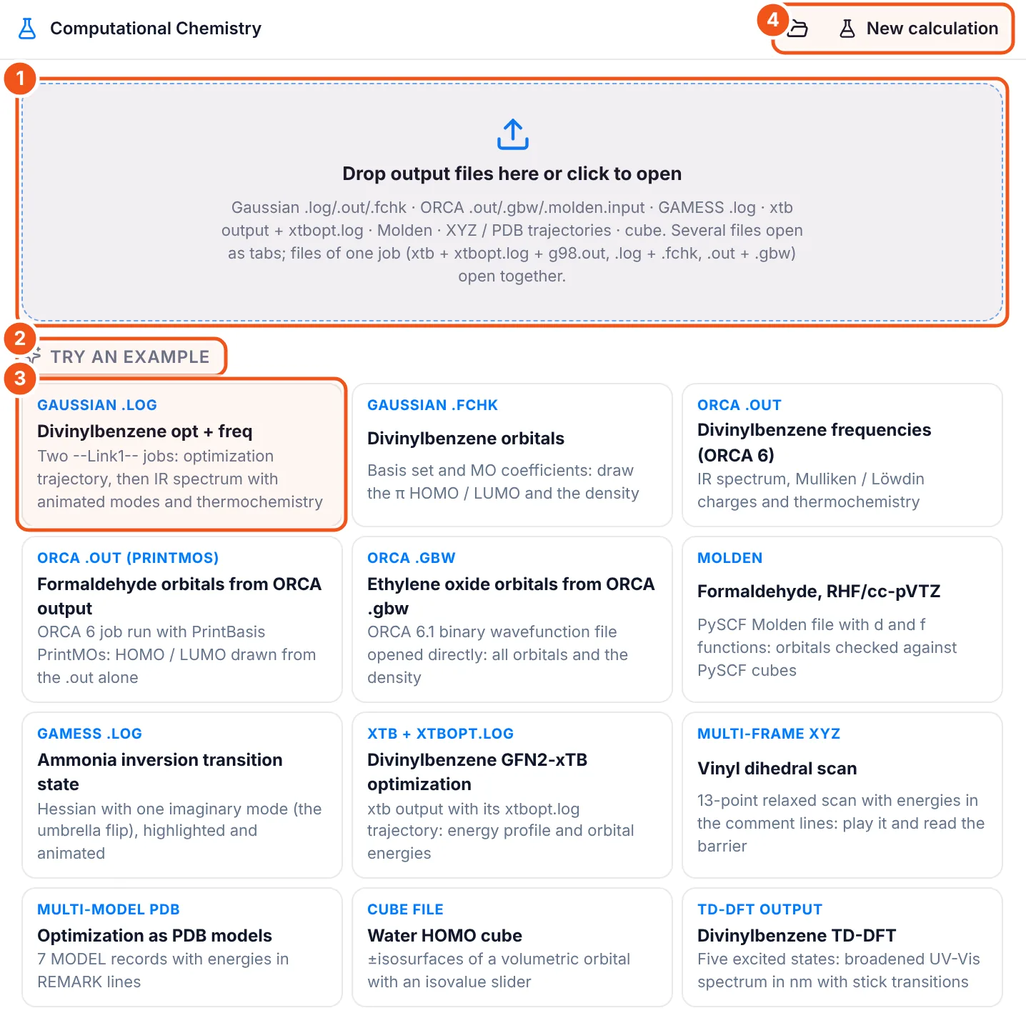
- Drop zone. Drag files here or click to choose them. Several files open as tabs; files from one job (for example
.log+.fchk, or.out+.gbw) open together in one tab. - Try an example: real outputs to explore before you use your own.
- Each card names the program and file type (here a Gaussian
.logwith an optimisation and a frequency job). - Open (folder icon) and New calculation, which builds input files (Step 8).
| Gaussian | .log / .out (including --Link1-- multi-job files) and formatted checkpoint .fchk. |
|---|---|
| ORCA | .out (orbitals with PrintMOs), binary .gbw and .molden.input. |
| GAMESS (US) | .log, including Hessians and transition states. |
| xtb | Output plus xtbopt.log for the optimisation path. |
| Molden | Geometry, basis and orbitals (including d and f functions). |
| Trajectories | Multi-frame XYZ (energies from the comment lines) and multi-model PDB. |
| Volumes | Gaussian cube files with ± isosurfaces. |
Files are read in your browser. Nothing is uploaded to a server.
Step 3: Read the key results (Summary)
We opened the example Divinylbenzene opt + freq (a B3LYP/STO-3G optimisation followed by a frequency job).
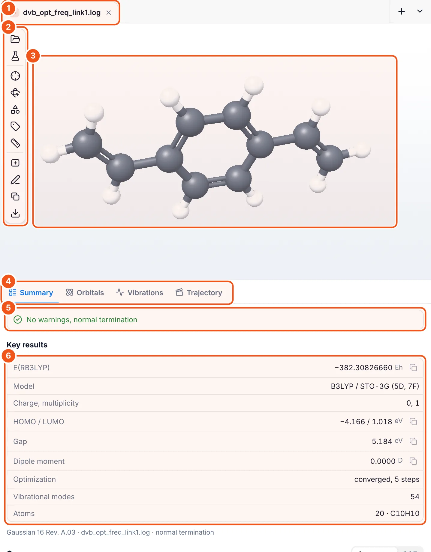
- File tab. Each open file gets a tab; the + on the right opens more.
- 3D toolbar: open, new calculation, fit view, spin, display style, atom labels, measure, add to canvas, send as a 2D drawing, copy image and export.
- 3D view of the final geometry. Drag to rotate, scroll to zoom.
- Result tabs. Only the tabs your file has data for appear: Summary, Orbitals, Vibrations, UV-Vis, Trajectory.
- Status: normal termination, or the warnings and errors found in the file.
- Key results: final energy (−382.30826660 Eh), method and basis, charge and multiplicity, HOMO/LUMO and gap, dipole moment, optimisation steps, number of modes and atoms. The copy icons copy single values.
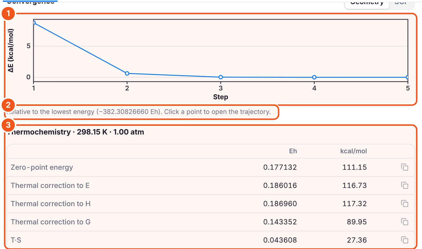
- Convergence of the optimisation (switch between Geometry and SCF). Click a point to open that step.
- Energies are relative to the lowest one, which is given in Eh.
- Thermochemistry at the temperature and pressure of the job: zero-point energy, thermal corrections to E, H and G, and T·S, in Eh and kcal/mol.
Step 4: Look at the IR spectrum and animate normal modes
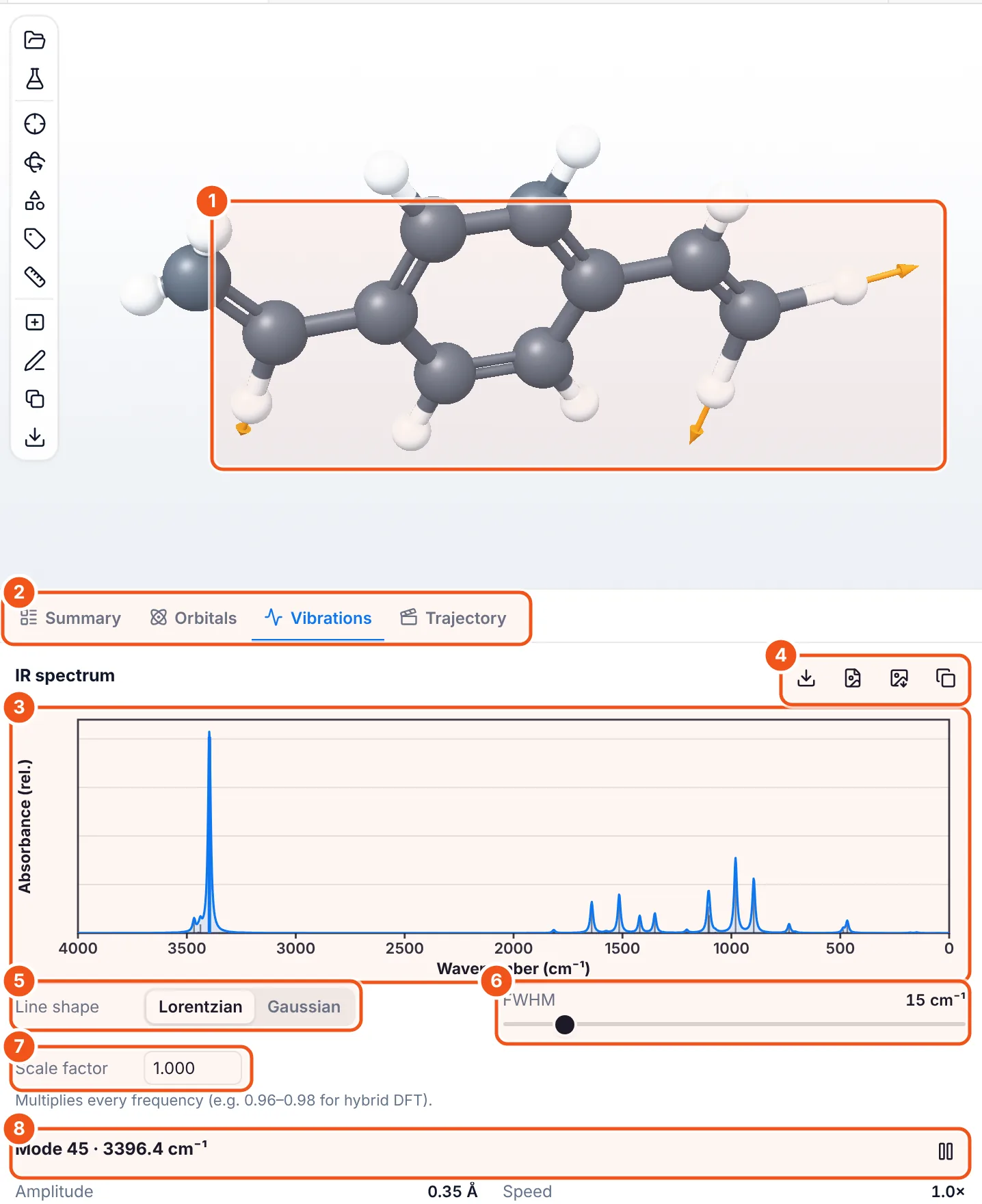
- The selected mode, animated, with arrows showing which way each atom moves.
- The Vibrations tab.
- The broadened IR spectrum. Click a peak or a stick to select its mode. When the file has Raman activities, an IR/Raman switch appears.
- Export as CSV (curve and sticks), SVG or PNG, and Copy image (see the tip below).
- Line shape: Lorentzian or Gaussian.
- FWHM: the peak width in cm⁻¹.
- Scale factor for the frequencies (for example 0.96 to 0.98 for hybrid DFT).
- The selected mode (here 45 at 3396.4 cm⁻¹, a C-H stretch). Below it: amplitude, speed and pause.
Tip for slides: the Copy image button (the last icon above the spectrum) puts the plot on your clipboard as a high-resolution PNG with a transparent background. Paste it straight into PowerPoint, Keynote or Google Slides; no file to save. The axes, numbers and labels are drawn bold so they stay readable on a projector.
Step 5: Draw molecular orbitals
Orbitals need the basis set and MO coefficients, so open a .fchk, .gbw, Molden file or an ORCA output with PrintMOs. We used the example Divinylbenzene orbitals (.fchk).
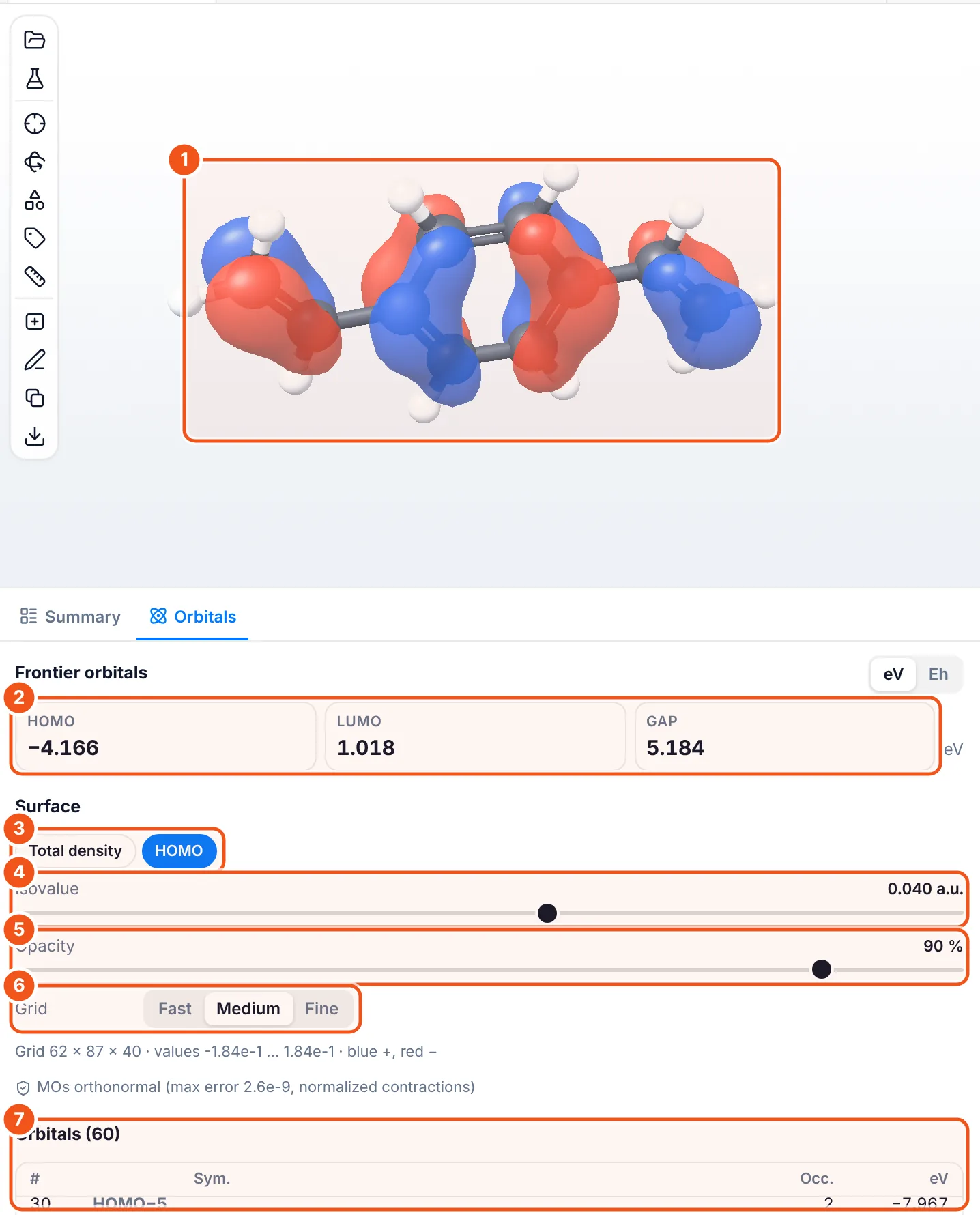
- The orbital surface on the molecule: blue for positive, red for negative.
- Frontier orbitals: HOMO, LUMO and gap, in eV or Eh.
- Surface: total electron density or the selected orbital.
- Isovalue: smaller values give bigger lobes.
- Opacity of the surface.
- Grid: Fast, Medium or Fine. Fine gives smoother surfaces and takes longer.
- The orbital table (here 60 orbitals) with symmetry, occupation and energy. Click any row to draw that orbital.
Under the grid line the panel checks that the orbitals are orthonormal, so you know the file was read correctly.
Step 6: Plot a UV-Vis spectrum from TD-DFT
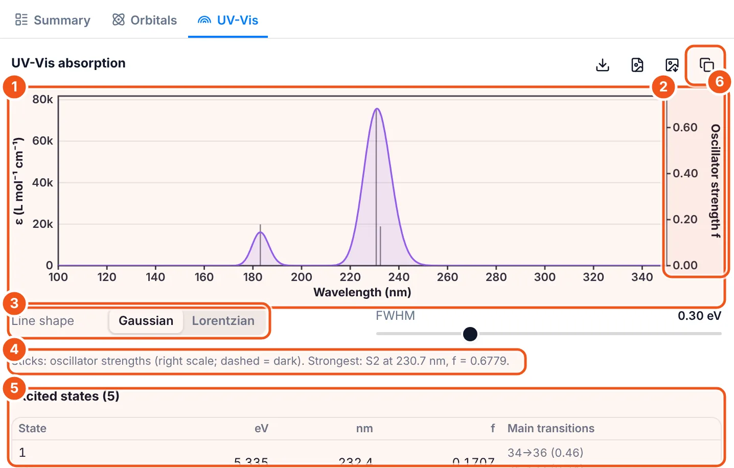
- The spectrum: ε (L mol⁻¹ cm⁻¹) against wavelength in nm, with each transition as a stick.
- The right axis gives the oscillator strength f of the sticks. Dark (forbidden) states are dashed.
- Line shape and FWHM (in eV).
- The strongest transition, here S2 at 230.7 nm with f = 0.6779.
- Excited states table: energy, wavelength, f and the main orbital transitions.
- Copy image: a transparent PNG for your slides. CSV, SVG and PNG export sit next to it.
Step 7: Play a scan or an optimisation
Multi-frame files play like a film. The example Vinyl dihedral scan is a 13-point relaxed scan of one vinyl group.
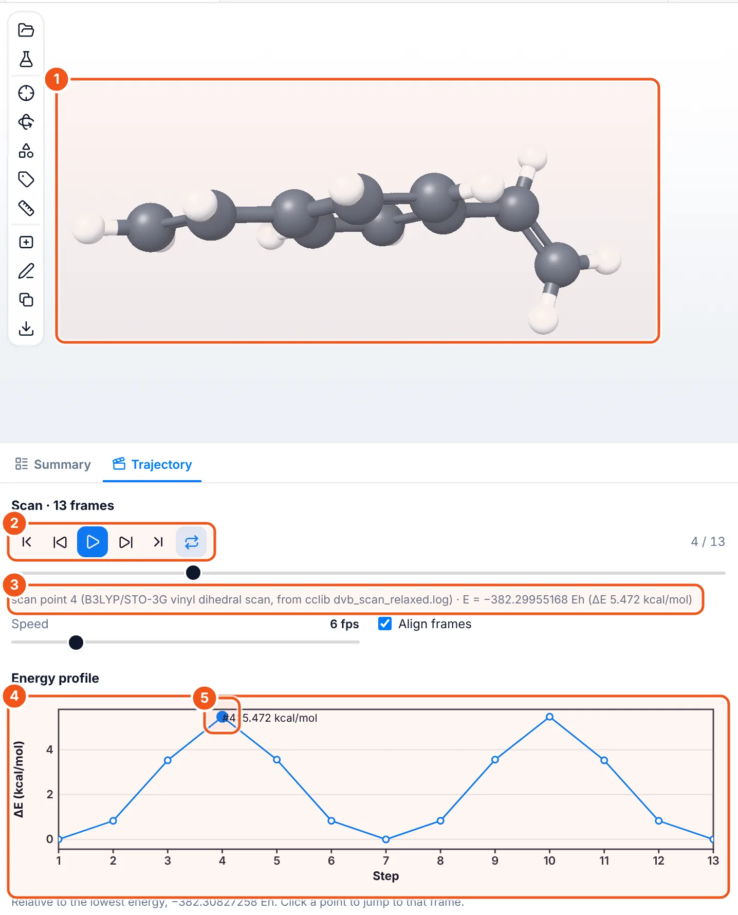
- The geometry of the current frame: at step 4 the vinyl group is twisted out of the ring plane.
- Player: first, previous, play, next, last and loop.
- The frame in words, with its energy and ΔE.
- Energy profile, relative to the lowest frame. Two barriers show the vinyl group passing the perpendicular position twice.
- The clicked point: frame 4, the top of the barrier at 5.472 kcal/mol.
Step 8: Make an input file for your next calculation
Click New calculation (flask icon). It takes the geometry from the open file or from your 2D drawing.
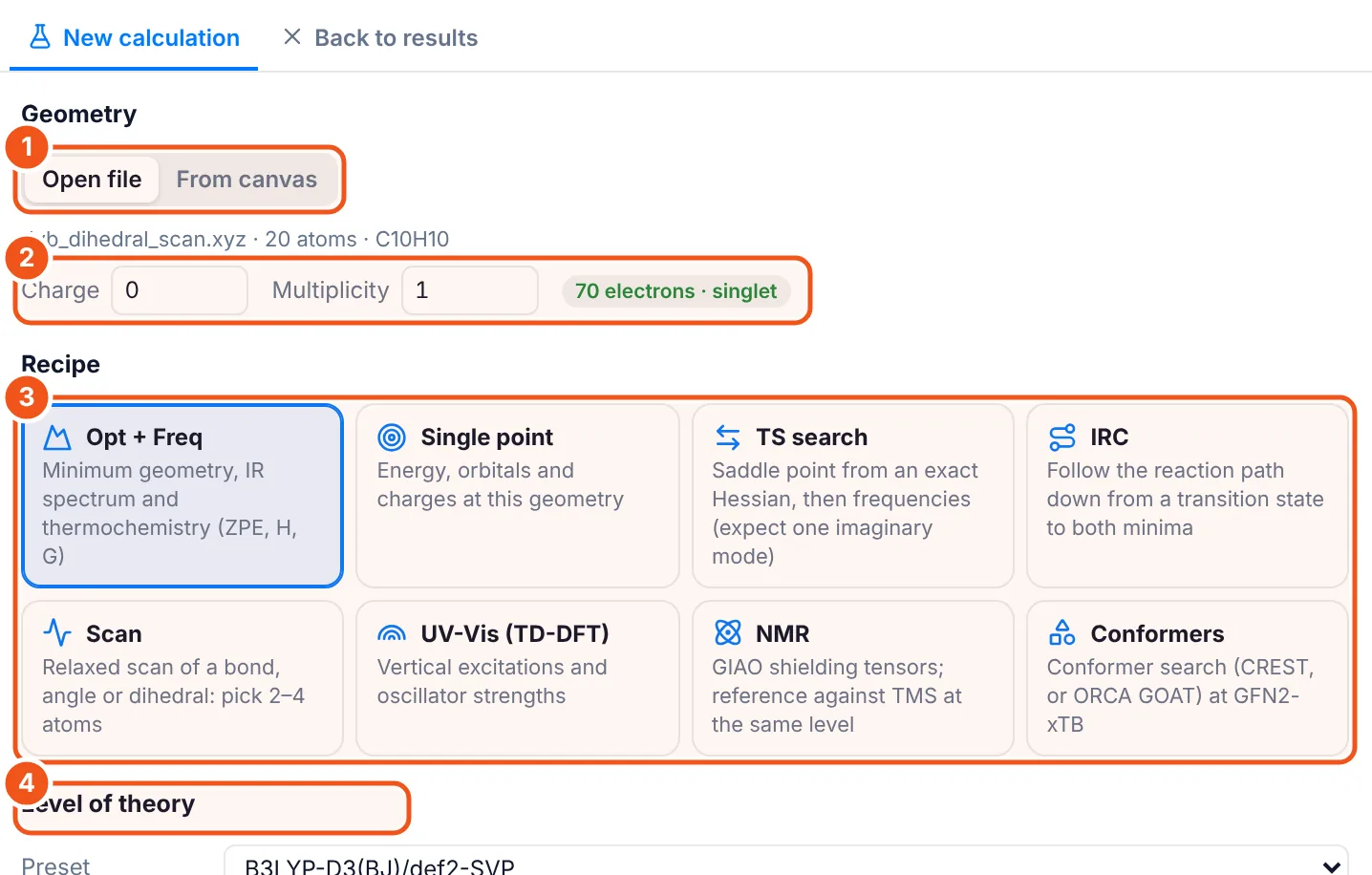
- Geometry from the open file or from the canvas.
- Charge and multiplicity, with an electron count check.
- Recipe: Opt + Freq, Single point, TS search, IRC, Scan, UV-Vis (TD-DFT), NMR or Conformers.
- Level of theory (next picture).
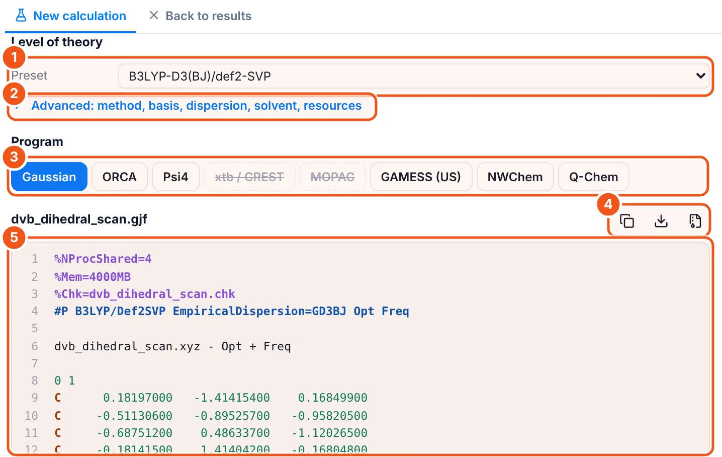
- Preset level of theory, here B3LYP-D3(BJ)/def2-SVP.
- Advanced: method, basis, dispersion, solvent and resources (cores, memory).
- Program: Gaussian, ORCA, Psi4, xtb/CREST, MOPAC, GAMESS (US), NWChem or Q-Chem. Programs that cannot run the chosen recipe are crossed out.
- Copy the input, download it, or download it with a run script.
- The generated input file with the route line, charge, multiplicity and coordinates.
When the job finishes, drop its output back on the panel to see the results.
Ways to use it
- Checking a job: see at a glance if it terminated normally, converged and has no imaginary frequencies.
- Teaching: animate normal modes, compare HOMO and LUMO, or play a torsion scan in class.
- Papers and talks: copy IR and UV-Vis plots as transparent images for slides, or export SVG for figures.
- Next step: build the next input from the result without retyping coordinates.
For predicted spectra without running a calculation, see the Spectroscopy plugin and the IR spectrum viewer.
Questions and answers
How do I open a Gaussian log file online?
Install the free Computational Chemistry add-on in MolDraw, open the CompChem tab and drop your .log or .out file on it. The file is read in your browser and is not uploaded.
Which programs and files are supported?
Gaussian .log, .out and .fchk; ORCA .out, .gbw and .molden.input; GAMESS (US) .log; xtb output with xtbopt.log; Molden files; multi-frame XYZ and multi-model PDB trajectories; and cube files.
How do I copy a spectrum into PowerPoint?
Click the Copy image button above the IR, Raman or UV-Vis plot. The plot goes to your clipboard as a high-resolution PNG with a transparent background; paste it into your slide.
Can I see molecular orbitals?
Yes, when the file has the basis set and MO coefficients: Gaussian .fchk, ORCA .gbw, Molden files or ORCA output with PrintMOs. Pick any orbital from the table and set the isovalue.
Can it write input files?
Yes. New calculation builds inputs for Gaussian, ORCA, Psi4, GAMESS (US), NWChem, Q-Chem, xtb/CREST and MOPAC from the open file or your drawing, for optimisations, frequencies, TS searches, IRC, scans, TD-DFT, NMR and conformer searches.
Is the Computational Chemistry add-on free?
Yes. You only need a free MolDraw account to install add-ons.